Calculus
\(\newcommand{\pd}[2]{\frac{\partial #1}{\partial #2}}\) \(\newcommand{\R}{\mathbb{R}}\) \(\newcommand{\RR}{\mathbb{R}}\) \(\newcommand{\C}{\mathbb{C}}\) \(\newcommand{\N}{\mathbb{N}}\) \(\newcommand{\Z}{\mathbb{Z}}\)
The core intution of calculus is that given a "nice" (analytic) function \(f : \R \to \R\), if I know it's value at some input \(x\), namely I know \(y\) for \(y := f(x)\), then I often want to know its value at \(f(x+\Delta)\), where \(\Delta\) is some very small number. If \(f\) were linear, this would be easy, because adding \(\Delta\) commutes with \(f\) in that case (i.e. \(f(x+y) = f(x)+f(y)\)).
For non-linear functions, we have instead:
This is the Taylor series, and the second term \(f'(x) := \lim_{\epsilon\to 0}\frac{f(x+\epsilon)-f(x)}{\epsilon}\) is the linear approximation of \(f\) at \(x\), known as the derivative of \(f\). \(f'(x)\) is also written as \(\frac{df(x)}{dx}\). This definition of the derivative requires limits, which makes the traditional approach to calculus rely on analysis (the study of limits and similar constructions on the reals).
The smaller \(\Delta\) is, the less the terms beyond the second one matter, which is to say that for small changes of the input, a locally linear approximation of \(f\) suffices for the correction term.
More generally, we should understand that if \(f\) is a function \(\R^n \to \R^m\), then at each point \(p\) in \(\R^n\), \(\frac{df}{dx}|_p\) is a linear function \(\R^n \to \R^m\) (and the second derivative is bilinear, and so on).
Taking the derivative is itself a linear operator, in the sense that (fixing a point \(p\)) it maps a function \(f\) to a new function \(\frac{df}{fx}|_p\), such that \(\frac{d(f+g)}{dx} = \frac{df}{dx} + \frac{dg}{dx}\).
Integrals
An integral is like a continuous analog of a sum, where you "count" the volume of a function. For example, \(\int_0^1 x^2 dx\) can be understood to be a continuous generalization, for \(f(x)=x^2\) of \(f(0) + f(0.1) + f(0.2) \ldots f(1)\).
Integration is a linear operator.
You integrate over a volume (in 1 dimension an interval of the real line, in 2, an area in \(\R^2\), etc).
The Riemann integral is one definition of integration (which coincides with the more general Lebesgue integration where both are defined). Take a function \(f:\R\to\R\) and consider an interval \([a,b]\subset\R\). Goal of integral is to find the area under the curve produced by \(f\). Consider any partition of \([a,b]\), i.e. a splitting up of \([a,b]\) into consecutive sub-intervals \(P_i\). You can define a piecewise constant function, \(g_P\), such that if \(x\in P_i\), \(g_P(x)=\inf_{y\in P_i}f(y)\), i.e. the lower bound of points in this stretch of \([a,b]\). It's easy to calculate the area under \(g\), because it's piecewise constant. Then you can try to find the partition \(P\) such that \(g_P\) has the largest area under the curve. The upper bound on how well you can do is \(L(f)=\sup_P \int_{[a,b]}g_P\). Note that this will result in your making your partition arbitrarily fine. Conversely we can dualize and consider \(U(f)=\inf_P \int_{[a,b]}h_P\), where \(h_P(x)=\sup_{y\in P_i}f(y)\). If \(U(f)\) and \(L(f)\) coincide, we say that \(f\) is Riemann integrable on \([a,b]\).
Note that \(L(f)\leq U(f)\), so showing the opposite inequality establishes equality and thus integrability.
All continuous functions are Riemann integrable.
Integration by parts
(if boundary term vanishes)
Analysis
Analysis is the careful building up of the concepts needed to talk about infinitesimal change. Not always a requisite for actually using calculus.
Sequence
A function \(S : \N\to B\) for some set \(B\) such as \(\R\) or \(\C^n\)
Series
A sequence T of the form \(T(n) = \sum_i^nS(i)\). Intuitively: the \(n\)th term of \(T\) is the sum of the first \(n\) terms of \(S\).
Cauchy Sequences, Convergent Sequences, and Completeness
A sequence \(S\) is Cauchy if \(\forall \epsilon>0:\exists k: \forall n,m > k: d(S(n),S(m))<\epsilon\)
A sequence \(S\) converges to a point \(p\) if \(\forall\epsilon>0:\exists k: \forall n>k: d(p,S(n))<\epsilon\)
A space is complete if all Cauchy sequences converge. Note: the reals, for example, are complete. The spaces in question can be more abstract - for example, the space of all Lebesgue integrable functions is complete. Here, we need a metric on functions.
Continuity:
Continuous function \(f: A\to B\) at a point \(x\in A\) is defined by:
Equivalently: a function \(f\) is continuous at a point \(x\) if \(\lim_{y\to x}f(y)\) exists.
Uniformly continuous function is defined as follows and is different from being continuous at every point:
Little o-notation
The statement \(f(x)=o(g(x))\) is a shorthand for: \(\lim_{x\to\infty}\frac{f(x)}{g(x)}=0\). This is very handy notation for discussing derivatives.
For example, consider \(f(x)=x^2\), and
Note that \(h^2\) in the numerator was not a linear function of \(h\), in particular, using little-o notation, we can say that \(h^2\) is \(o(h^n)\) for \(n>2\), and as such drops out.
This pattern crops up all the time, where to find the derivative of a function, you can drop all terms that are \(o(h^n)\) for \(n>2\). In particular, it's used in the context of Taylor series expansions, e.g. you could write: \(e^x=1+x+o(x^2)\).
Taylor Series
A power series representation of \(f(x)\) takes the form \(\sum_{i=0}^{\inf} c_i(x-a)^i\). What's cool is that if such a series exists for an infinitely differentiable function \(f\), we can recover the "basis coefficients" \(c_i\) by noting that: (1) \(f(a) = c_0\) and (2) that \(f'(x) = \sum_{i=1}^{\inf} ic_i(x-a)^{i-1}\), so that \(c_1 = f'(x)/1\). Continuing in this vein with \(n\)th derivatives, we find that \(c_i = \frac{d^{(i)f(x)}}{dx^{(i)}}(a)\frac{1}{i!}\). Substituting in these values for \(c_i\) into the series gives us the Taylor series.
$$ T(f)(t_0)(t) = \sum_{i=0}{\infty}\frac{f(t-t_0)^i $$ The intuition is that for a point }}{i!\(x\), we're approximating \(f\) locally by a sum (which when infinite may converge to a perfect approximation) of the derivatives of \(f\) around that point. This makes sense: the derivatives give you local context: first derivative is what the function is doing nearby, second derivative is what the first derivative is doing nearby, etc.
Example
Write \(f(x+a)=f(x)+af'(x)+\frac{a^2}{2}f''(x)...\). Then note that to find the second derivative, we can write:
Here the approximation becomes increasingly precise in small \(a\), i.e. the error is \(o(a^2)\).
A natural extension to \(\C\), \(\R^n\) and \(\C^n\) exists. The Taylor series up to term \(n\) is the \(n\)th order approximation of \(f\), which is a polynomial. Write it as \(T_n(f)(t_0)\).
It is often useful to ask about the remainder \(R_n(f)(t_0)=T_n(f)(t_0)\).
Taylor's theorem states that \(R_n(f)(t_0)(t)=o(|t-t_0|^n)\) as \(t_0\to t\). In other words, for \(t_0\) sufficiently close to \(t\), the error is dominated by a polynomial of order \(n\).
We can also give explicit formulas for the remainder, such as the integral form:
From which the mean value theorem gives us that:
Here \(t'\) is known to exist by the mean value theorem.
Some examples of integrals
First note that \(d(a\cosh y)=a\sinh y dy\) and that \(\cosh^2 y-1=\sinh^2 y\). Then make the substitution in the integrand: \(x=a\cosh y\). Simplifying:
Multivariate Calculus
These are results at the intersection of linear algebra and calculus.
One of the really important ideas is that the differential \((Df)(x)\) of a function \(f\) \(\R^n\to\R^n\) is a linear map. This is one of the reasons why linear algebra is so important.
The derivative of \(f:\R^n\to\R^n\) at a point \(p\) is the limiting linear approximation of \(f\) given by the line between \(p\) and \(q\) as \(q\) nears \(p\). In the general multivariate case, the differential \(Df:\R^n\to L(\R^n\to\R^n)\), if it exists, is a linear map characterized by: $$ \lim_{x\to a}\frac{||f(x)-f(a)-Df(a)(x-a)||}{||x-a||} = 0 $$ or equivalently $$ \lim_{x_0\to 0}\frac{||f(a+x_0)-f(a)-Df(a)(x_0)||}{||x_0||} = 0 $$ So basically the idea is: the total derivative \(Df(a)\) is the limiting linearization of \(f\) around \(a\).
The following is also true (using index notation):
Chain rule
Or without index notation:
Gradient \(\nabla\) and Hessian \(H\)
Examples:
Change of variables
The idea is that instead of integrating \(f\) with respect to its input \(x\) (i.e. calculating \(\int_Af(x)dx\)), we can view \(x\) as a function of \(u\) (i.e. \(x=g(u)\)) and then pull back to an integral over \(u\) (i.e. \(\int_{g^{-1}(A)}f(g(u))du\)). But this is a differently valued integral. So this new integral requires a term to offset the change, which rather nicely happens to be \(|Det(D_ug(u))|\). The intuition is that we account for the change in area of the differential (as it approaches the limit). The absolute value is because the sign of the determinant only measures the order of the dimensions and we don't care about this here. The equation looks as follows:
where \(Dg(x)\) is the determinant of the matrix of partial derivatives of \(g(x)\) wrt. \(x\).
Arguments with differentials
It's often very handy to reason in terms of small elements, which you then take to \(0\) in the limit. For example, suppose \(y(x)\) is the height of a curve. Then consider a section of width \(\Delta x\) which starts at a point \(x\), and note that its length is \(((\Delta x)^2+(y(x+\Delta x)-y(x))^2)^{\frac{1}{2}}\). Dividing by \(\Delta x\), we obtain:
Because limits can go inside continuous functions, we can say that:
Derivative of the determinant
Existence and Differentiability of the Matrix Exponential
\(e^{t\psi}=\sum_{i=0}^{\infty}\frac{t^i\psi^i}{i!}\). The series is Cauchy, since \(||\sum_{i=0}^{m+1}\frac{t^i\psi^i}{i!}-\sum_{i=0}^{m}\frac{t^i\psi^i}{i!}||=||\frac{t^{m+1}\psi^{m+1}}{(m+1)!}\leq \frac{t^{m+1}}{(m+1)!}||\psi||^{m+1}\), which is dominated by the factorial term. Thus the sequence converges (the space of linear operators being complete).
Differentiability of \(f(t)= e^{t\psi}\):
\(\frac{d}{dt}f(t)=\lim_{h\to0}\frac{1}{h}(e^{(t+h)\psi}-e^{t\psi})=\lim_{h\to0}(e^{h\psi}+I)e^{t\psi}\)
So all that it needed is to show that \(\lim_{h\to0}(e^{h\psi}+I)=\psi\).
We can then rather cleverly observe that the this final sum goes to \(\psi\) as we take \(t\) to \(0\), because the term of the sum with \(i=0\) is \(\frac{0^0\psi}{0!}=\psi\).
Non-linear dynamics
Note
This section is based on Strogatz's Nonlinear Dynamics and Chaos, and was cowritten with Sandra Romero Pinto.
In general, we're interested in functions \(x : \mathbb{R^n}\to\mathbb{R^m}\) satisfying some differential equation \(x'(t)=f(x(t))\), so that their local linearizations at a point are linear maps also of \(\mathbb{R^n}\to\mathbb{R^m}\). Note that this is a first order differential equation, but higher order ones can be reformulated as first order by considering \(x, x', x''...\) as a vector of variables.
When \(f\) is a linear map, the solution takes the form \(e^{ft}\) and everything is nice, because linear algebra provides powerful tools that are applicable in this case. But when \(f\) is not a linear map, things can be hard. Calculus provides a powerful tool for handling non-linear systems, namely that the first order approximation of a non-linear system is linear. Sometimes the linear approximations tell you everything important about the non-linear system (see the Hartman-Grobman theorem). Often, however, even this isn't enough.
When it isn't, one can instead study the fixed points, which are points \(x^*\) where \(f(x^*)=0\), called as such because if you start at such a point, you stay at it.
There's an intuitive notion of stability of fixed points, namely whether arbitrarily small pertubations of a fixed point result in a return to the fixed point (stable) or not (unstable).
Fixed points are a sort of topological feature of an ODE, in the sense that we can qualitatively characterize a solution by asking about the number and stability of its fixed points, rather than finding the exact value of \(x\) at all \(t\).
This leads naturally to the notion of a bifurcation, where you have an ODE parametrized by some parameter \(p \in \mathbb{R}\) and as you vary \(p\), you find that at some point the number or stability of the fixed points changes. This is a bifurcation.
Linear Stability Analysis
We can be clever about analyzing stability by forming a new ODE in terms of a perturbation around a fixed point. That is, for a fixed point \(x_0\), and in the 1D case:
Then it follows that:
This final approximation is true for \(f'(x^*)\neq 0\) in the limit of small \(\eta\). Solving this ODE (\(\dot{\eta}=\eta f'(x_0)\)) shows that for \(f'(x_0)>0\), the perturbation grows, and for \(f'(x_0)<0\) is shrinks, returning the trajectory back to the fixed point. For \(f'(x_0)=0\) we're back to square one.
This generalizes to the n-dimensional case (see these ODE notes), where \(f'\) becomes the Jacobian. Then, the case of all eigenvalues with negative real part gives stability, all positive real part gives instability. More generally if all eigenvalues have a real part, this is known as a hyperbolic fixed point. The cases where at least one eigenvalue has real part \(0\) are the difficult ones, as the linearization around a fixed point doesn’t always reflect the true phase portrait of the non-linear system
Definitions to describe stability of fixed points (linear/nonlinear)
Considering \(\textbf{x}^*\) the fixed point of a dynamical system:
- \(\textbf{x}^*\) is an attracting point if $x(t) \to \textbf{x}^,\text{as}, t \to \infty $ (trajectories starting near it eventually converge to \(\textbf{x}^*\)) . It can be called *globally attracting if it attracts all trajectories (but sometimes it has a certain basin of attraciton. Focuses on the condition of \(t \to \infty\)
- \(\textbf{x}^*\) is a Lyapunov stable: if trajectories starting sufficiently close to \(\textbf{x}^*\),remain close to it at all times.
A given \(\textbf{x}^*\) can be both attracting and Lyapunov stable, or only either.
- \(\textbf{x}^*\) can be attracting but not Lyapunov stable: if trajectories actually diverge from the fixed point to then converge on it as $t \to \infty $ (no particular name for this)
- If it’s only Lyapunov stable then \(\textbf{x}^*\) is neutrally stable: trajectories remain near it but never actually converge on it.
- If it’s both, \(\textbf{x}^*\) is asymptotically stable
- if it’s neither, \(\textbf{x}^*\) is unstable
1D ODEs
For \(x : \mathbb{R}\to\mathbb{R}\), the kinds of solutions are limited (all solutions either approach a fixed point or diverge to \(\pm\infty\), as are the kinds of birfurcations.
The following is a list of the kinds of birfurcations in 1D. For each kind, I list the normal forms. These are simple ODEs which provide an example of the kind of bifurcation, but note that not all bifurcations are of the normal form. For example, \(\dot{x}=-x + \beta\tanh x\) has a saddle node bifurcation. However, to a first order approximation (i.e. locally) the normal form is equivalent to any other bifurcation of that class.
Normal forms are therefore the 1st order approximation to all these canonical bifurcations. Here are the 1D normal forms:
- saddle-node bifurcations: at which the number of fixed point changes
- normal forms: \(x^2 - r\) and \(x^2 + r\)

- transcritical bifurcations: at which the fixed points change their stability
- normal forms: $ rx - x^2$

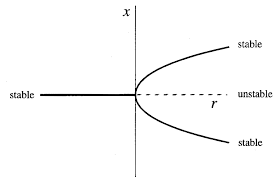
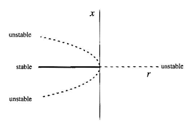
- pitchfork bifurcations: number of fixed point changes but also the stability changes (...). The core feature is that the system has symmetry (it behaves the same if \(x\mapsto -x\) ). Can be sub-or supercritical depending on the stability of the remaining fixed points after the bifurcation (the names are counter-intuitive for the stability of the remaining fixed points)
- supercritical normal form: \(rx - x^3\)
- subcritical normal form: \(rx + x^3\)
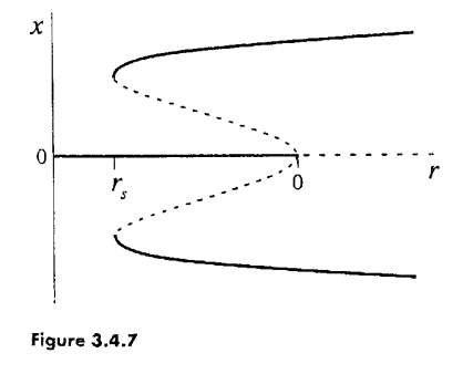
- subcritical with hysteresis: \(rx + x^3 - x^5\)
As an example of a complicated ODE which takes a well-known normal form in the 1st order, consider:
For \(u := x -1\), \(\dot{u} = r\ln(1+u)+u = r[u-\frac{1}{2}u^2 + O(u^3)] + u = (r+1)u - \frac{1}{2}ru^2 + O(u^3)\). Up to rescaling, this is the normal for for a supercritical pitchfork bifurcation.
Usefulness of graphs
Stability of a fixed point can be determined by just looking at the vector field of the system: in a 1D system, this is given by an \(\dot{x}\) against \(x\) graph.
Points crossing the x-axes are the fixed points and the stability can just be determined by looking at the sign of \(\dot{x}\) around that fixed point (basically checking whether x would approach or diverge from that fixed point given the sign of the derivative \(\cdot{x}\)).
2D ODEs
Some common kinds of fixed points include:
Limit cycles
They are closed & isolated trajectories, meaning that the trajectories neighboring it are not closed but are spirals toward (stable limit cycle) or away (unstable limit cycle) to /from it. Sometimes they can be half-stable (toward or away from it inside or outside of the closed trajectory) . They are inherent of nonlinear systems, as closed orbits in linear systems can’t be isolated by the definition above, and in contrast form families of closed orbits whose amplitude is scaled by a constant (determined by the initial conditions and preserved, there can never be spirals in linear systems).
Limit cyles can’t exist if a Lyapunov function exists for the system. Intuitively, this is an energy-like function that decreases along trajectories. More formally: it’s a continuously differentiable real-valued function \(V(\textbf{x})\) that : 1) is positive definite : \(V(\textbf{x})>0 ~ \forall \textbf{x} \neq \textbf{x}^* , V(\textbf{x}^*)=0\) , 2) for which all trajectories go downhill in the V function towards \(\textbf{x}^*\) : \(\dot{V}<0 ~ \forall \textbf{x} \neq \textbf{x}^*\).
Focusing on property 2) this would make the fixed point to be globally stable (all trajectories move towards is) and would make it impossible to have a closed trajectory (i.e. limit cycle) as this would imply that \(\dot{V} =0\).
Other ways of ruling out limit cycles are by determining whether the system is gradient system (very similar to figuring out whether a Lyapunov function exists), and Dulac’s criterion. The Poincaré-Bendixson theorem is used to determine whether a closed orbit exists in a system.
Bifurcations
All the 1D cases still apply, but there are now some more cases too. In 1D, eigenvalues lie on the real line, but in 2 or more dimensions, they can be complex. In particular, for 2D, the eigenvalues are the solution of a quadratic equation with real coefficients (see linear algebra notes), so if \(4ac\) is non-negative, they are both real, and if \(4ac\) is negative, they are both complex conjugates (because \(\sqrt{4ac}\) is purely imaginary, it's negative is its conjugate, and then the other terms of the quadratic formula shift and scale along the real axis).
So now we have a new case, where the change of stability occurs when both eigenvalues cross the imaginary axis at once. These are Hopf bifurcations.
Chaos
The original and typical example is the Lorenz equations. These are a 3D ODE whose long term behavior is not convergence to a fixed point or limit cycle, but is confined to a bounded region. Note that this would violate Poincaré-Bendixson in 2D. The surprising conclusion is that the long-term behavior converges to a strange attractor, which is a set of measure \(0\) not unlike the Cantor set.
Functional derivatives
Particularly in physics, the word functional is used to mean a function of type \((\R^n \to \R^n) \to \R\). Why they need a special word for this (or square brackets for its arguments) is unclear. At any rate, one can define derivatives of functionals as:
To see that the types make sense, view \(f\) as an infinite dimensional vector; as in the finite case, for \(F : \R^n \to R\), we have \(\frac{\partial F(f)}{f} : \R^n\). So for \(n=\infty\), \(\frac{\partial F(f)}{f}\) is itself a function.
Note that we characterize \(\frac{\partial F(f)}{f}\) by its inner product, or action on \(g\). This is much like the theory of distributions in Fourier analysis.
Two common cases. First:
And second:
Calculus of variations
A subdomain of functional analysis concerns finding minimal functions, and predates the more general field by quite some time (i.e. goes back to Newton).
Note that the word variational, as in variational bound or variational inference refers to the calculus of variations.
Here's a helpful perspective. View a vector as a function \(A\to\R\) for \(A\subset \Z\), i.e. a map from indices of the ``array'' to the value at that index. Then the continuous version is a natural extension.
Roughly, the first functional derivative, analogous to the first derivative for ordinary calculus, where \(\eta\) is some other function with the same support, looks like:
A particularly important type of functional in physics and elsewhere takes the following form, for \(L : \R\to\R\to\R\to\R\):
It turns out that minimizing such a functional (or more generally finding values of the function \(x\) for which \(\partial A_L(x)=0\)), which you might imagine to be totally totally intractable, is not so hard (terms and conditions apply). This is because whenever \(x\) is such that \(\partial A_L(x)=0\), the following partial differential equation (called the Euler-Lagrange equation) is also true:
Derivation of Euler-Lagrange
For a function \(f\), let \(\delta f\) denote a variation of the function. Note that linearity and the chain rule operate in a normal sort of way. As before, \(A_L(x) = \int_a^b L(t,x(t),x'(t)) dt\).
We now integrate the second term by parts, noting that \(\delta x(a)=\delta x(b)=0\) (this is part of the definition of a variation), to obtain:
If \(\delta A_L=0\), then \(\frac{\partial L}{\partial x} - \frac{d}{dt}\frac{\partial L}{\partial x'}\) must also be \(0\) (since anywhere where it was not \(0\), you could choose \(\delta x\) to be non-zero in only that region, and then \(A_L\) would no longer be \(0\)).
Example of use of Euler-Lagrange equation:
\(L(x,y(x),y'(x)) = \sqrt{1+y'(x)^2}\)
Arc length: \(F_L(f) = \int_a^b L\)
The Euler-Lagrange equation gives us:
$$0 = - \frac{d}{dx}\frac{\partial\sqrt{1+y'(x)^2}}{\partial y'(x)} = \frac{d}{dx} \frac{y'(x)}{\sqrt{1+y'(x)^2}} $$ So
For \(A := \sqrt{\frac{C^2}{1-C^2}}\), \(y'(x) = A\), so that \(y(x)=Ax+B\).
What we have shown: the function which minimizes arc length is a straight line. Good to know...
Technically we also have to impose some conditions on the second derivative, as in the normal case of minimization.
Stirling's Approximation
\(N!\) rapidly becomes intractable to analytically or numerically compute, which is bad for statistical mechanics, because it appears a lot. But for large \(N\) we can estimate it. First a rough estimate, and then a better one:
More
A second, better approximation is attained as follows, recalling that \(\Gamma(n)=n!\) for \(n\in \Z\), where
We then do something crazy, which is to approximate the integrand by a Gaussian. The reason this works well is that the integrand \(f(x)=e^{-x}x^N\) is peaky. The gaussian function is:
We set the mean \(x_0\) at the maximum, which is found by setting \(0=\frac{d}{dx}\log e^{-x}x^N=\frac{d}{dx}N\log x-x=\frac{N}{x}-1\), which implies that \(x_0=N\). Then \(A=g(x_0)=g(N)\approx e^{-N}N^N\).
Finally, we note that \(\frac{d^2}{d x^2}\log g(x)=-\frac{1}{\sigma^2}\) and equating this to \(\frac{d^2}{d x^2}\log f(x)=-\frac{N}{x^2}\) implies that \(\sigma\) should be set to \(\frac{x^2}{N}\)
This gives: