Tensor Networks

Assumptions

Here I assume the reader is familiar with the basics of probability theory and tensor networks.

References

• Quantum Field Theory and Condensed Matter

• Some great notes from Miles Stoudenmire.

• Ising Gauge Theory

The goal here is to explain the relationship between tensor networks and the Ising model.

The Ising model is really just a Markov random field with a 2D square lattice topology. It is therefore a classical probability distribution, on the Cartesian product of \(L_xL_y\) boolean variables, where \(L_x,L_y\) is the width (resp. height) of the lattice. The normalization constant (partition function) is given by:

\[ Z_{cl}(K_x, K_\tau) = \sum_s e^{\sum_i K_xs_is_{i+x} + K_\tau(s_is_{i+\tau} - 1)} \]

where \(s_i, s_{i+x}\) are horizontal neighbours and \(s_i, s_{i+\tau}\) are vertical neighbours, the sum is over all possible configurations of the boolean variables (spins, as physicists call them), and \(K_x, K_\tau\) are parameters. \(\beta\) is set to \(1\). The \(-1\) in the second term doesn't change the physics, but is convenient for the derivations below.

The Ising model as a quantum system

As is often the case, we can also find a quantum system with Hamiltonian \(H_q\) with a canonical partition function that is the same as the classical system we started with. Concretely, \(Tr[(e^{- H_q})^{L_y}] = Tr[e^{- L_yH_q}] = Z_{cl}\), with:

\[ H_q(K_x,K_\tau) = -\sum_i b(K_\tau) \sigma_1(i) + K_x\sum_i \sigma_3(i)\sigma_3(i+1) \]

where \(\sigma_3(i) := I_1 \otimes \ldots \otimes I_{i-1} \otimes \sigma_3 \otimes \ldots I\), \(K\) is a parameter, and \(b(K) = \tanh^{-1}(e^{-2K})\). This is the transverse Ising model.

A state in the transverse Ising model lives in the Hilbert space \(\bigotimes_i^N \mathbb{C}^2\). As you'd expect, the classical states of a single site \(i\) are the eigenvalues of \(\sigma_3(i)\).

Note

\(b\) is an involution, and is related to the Kramers–Wannier duality. Taking the simplest case of \(K_\tau = K_x := K\), note that each choice of \(K\) yields a transverse Ising model, which yields a classical Ising model, which is a distribution. So we can think of \(K\) as the coordinates on a manifold of distributions. The duality is simply that \(K\) and \(b(K)\) denote the same distribution, or more precisely:

\[ \frac{Z(K)}{(\sinh 2K)^{\frac{N}{2}}} = \frac{Z(b(K))}{(\sinh 2b(K))^{\frac{N}{2}} } \]

This can be seen by the fact that for the Hamiltonian, \(-\sum_i b(K) \sigma_1(i) + K\sum_i \sigma_3(i)\sigma_3(i+1)\), \(K \mapsto b(K)\) is the same as switching \(\sigma_1(i)\) and \(\sigma_3(i)\sigma_3(i+1)\), which is how the duality is usually presented.

Derivation

We want to show that \(Tr[e^{-L_y H_q}] = Z_{cl}\).

Define:

\[ V_1 := \frac{e^{\sum_i^N b(K)\sigma_1(i)}}{\cosh^N b(K)} \\ \quad \quad \quad \\ V_3 := e^{\sum_i K\sigma_3(i)\sigma_3(i+1)} \]

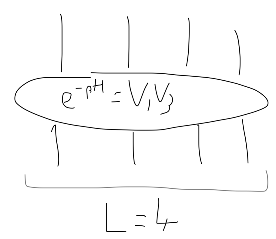
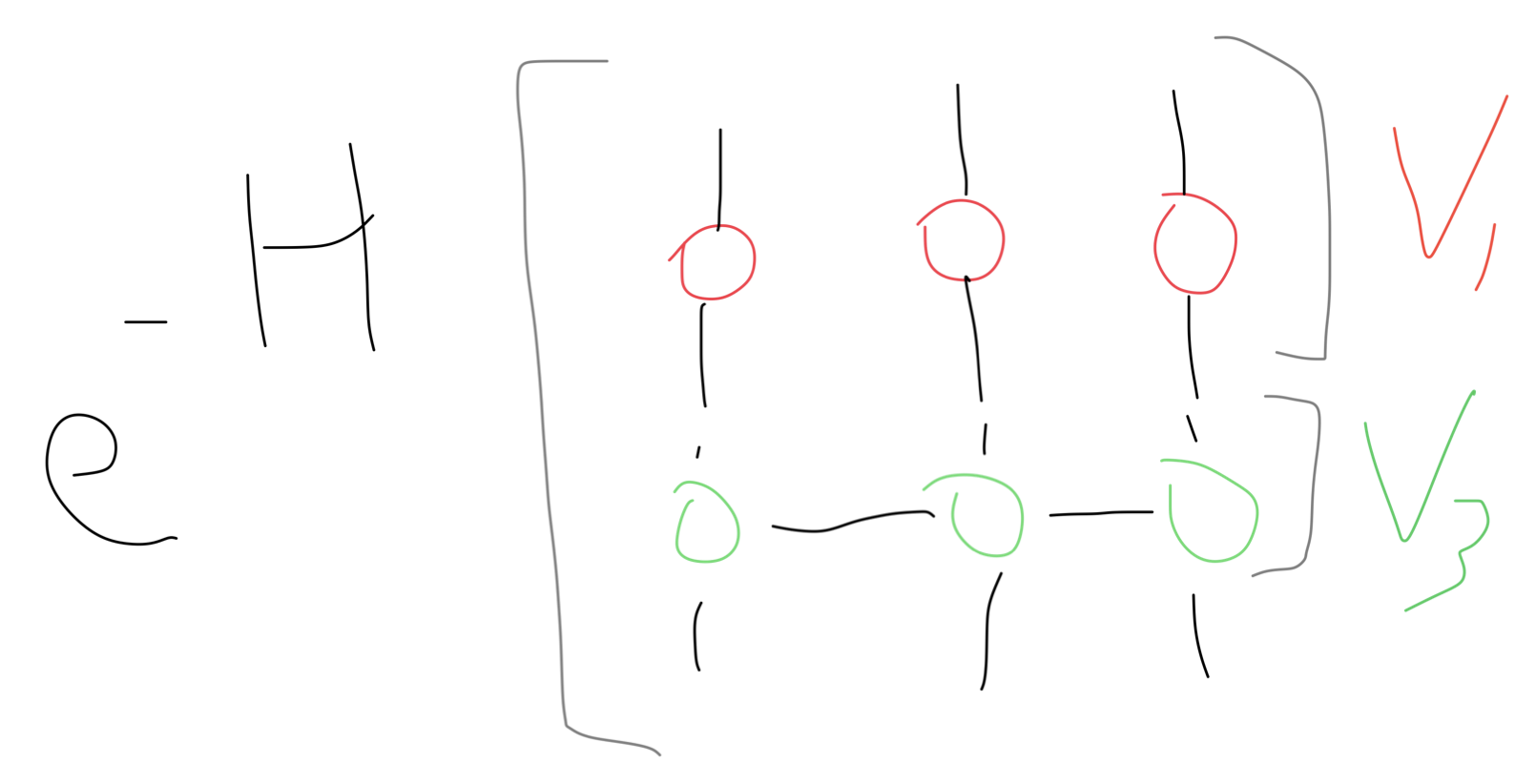
so that \(e^{-H_q - C}=V_1V_3\) for some constant \(C\).

We then calculate \(\langle s'|V_1V_3|s\rangle\) for two states \(s, s'\) that are both eigenvectors of all \(\sigma_3(i)\):

\[ \langle s' | V_1V_3 | s \rangle \\ = \langle s' | V_1| s \rangle e^{\sum_i Ks_is_{i+1}} \\ = \prod_i^N\langle s_i' | \frac{e^{\sigma_1(i)}}{\cosh b(K)}| s_i \rangle e^{\sum_i Ks_is_{i+1}} \]

\[ = \prod_i\langle s_i' | \frac{\cosh b(K) I + \sinh b(K)\sigma_1(i)}{\cosh b(K)}| s_i \rangle e^{\sum_i Ks_is_{i+1}} \]

\[ = \prod_i\langle s_i' | I + \tanh b(K)\sigma_1(i)| s_i \rangle e^{\sum_i Ks_is_{i+1}} \]

\[ = (\delta_{s_i, s'_i} + \delta_{s_i, -s'_i}e^{-2K})e^{\sum_i Ks_is_{i+1}} \]

Observe that for \(L_y=1\), \(Tr[e^{-L_yH_q}]=\sum_{s,s'}\langle s' | V_1V_3 | s \rangle\), which is what we just calculated, and is evidently equal to the classical partition function \(Z_{cl}\). The result extends to \(L_y=n\) in an obvious way.

Graphically, we have \(e^{-H_q}\):

The Ising model as an MPO

The next observation is that \(e^{-H_q}\) is actually an MPO, that is:

This is easy to show. Recalling that \(\exp(i\theta v\cdot \overrightarrow\sigma) = \cos(\theta)I + i\sin(\theta)v\cdot \overrightarrow \sigma\), observe that \(e^{i\sum_j^N (-ib(K))\sigma_1(j)} = \prod_j e^{i(-ib(K))\sigma_1(j)} = \prod_j(\cos(ib(K))I + \sin(ib(K))\sigma_1(j))\) which is just a tensor product of 2x2 matrices. Similarly, \(e^{i\sum_j (-iK)\sigma_3(j)\sigma_3(i+1)} = \prod_j e^{i(-iK)\sigma_3(j)\sigma_3(i+1)} = \prod_j(\cos(-iK)I + i\sin(-iK)\sigma_3(j)\sigma_3(i+1))\), which is an MPO.

To calculate \(Z_{cl}\), we then contract the MPO against itself repeatedly.

Defects (Excitations)

One can then study variations to this tensor network, such as the effect of interposing a 1D tensor network in the middle of the Ising TN.

For physical reasons, these are called defects, and have an algebraic structure that has come up a lot in recent theoretical quantum condensed matter physics.

I believe they form a fusion category, isomorphic to the category of representations¹ of some Lie group, maybe \(SU(2) \times SU(2)\)?

Under construction...

---

1. That is, a category where the objects are irreducible representations (i.e. functors from a given group to the category of vector spaces) and the morphisms are natural transformations between these functors, which amount to linear maps satisfying an intertwining condition. This category has a monoidal product and a direct sum, both inherited from linear algebra. Rules for e.g. addition of angular momentum, which is about the direct sum decomposition of the monoidal product of irreps are, I think, the fusion rules of the category. ↩