Statistical Physics
\(\newcommand{\pd}[2]{\frac{\partial #1}{\partial #2}}\) \(\newcommand{\R}{\mathbb{R}}\) \(\newcommand{\Z}{\mathbb{Z}}\) \(\newcommand{\RR}{\mathbb{R}}\) \(\newcommand{\C}{\mathbb{C}}\) \(\newcommand{\N}{\mathbb{N}}\)
Note
These notes are strongly opinionated, following Jaynes, and present statistical physics as the application of the maximum entropy principle to physical systems. Furthermore, thermodynamics is presented in terms of the geometry of the information manifold, following Caticha.
This seems like the natural modern approach, since it demystifies entropy, temperature and so on, viewing them as information-theoretic concepts, and not intrinsically physical ones. On this view, statistical physics is not new physics, it is the application of probability theory to old physics.
However, note that it isn't entirely uncontroversial, and a common criticism is that it makes temperature dependent on the information state of an observer, rather than being a property of the system. I take the view that this is indeed the case, but see Caticha for nuanced discussion.
Statistical physics
Statistical physics examines systems up to incomplete information, using the standard apparatus of Bayesian probability theory. That is, we describe our (incomplete) knowledge of a system by a probability distribution over systems, \(p : Dist(Time \to C)\), where \(C\) is the configuration space of the system, classical or quantum.
While systems live on one manifold (the microspace), the space of interest to statistical physics (call it the "macrospace") is the manifold of distributions over the original space. Each macrostate is really a whole distribution over microstates. Quantities of interest, like energy, can be viewed as expectations over the distribution.
Often the macrospace is much lower dimensional than the microspace (when we only consider maximum-entropy distributions - see below). This is why statistical physics is so effective.
Note
It is important to note that statistical physics often involves very large systems (e.g. a system of \(10^{23}\) particles), but doesn't need to. It makes total sense to consider a distribution over a single particle system. It is just that many common results do not hold in this situation, but all the ensembles are defined exactly the same.
Note
The language in which statistical physics is usually expressed is frequentist. That is, an ensemble is described as being "many copies of a system". The Bayesian way to think, followed here, is not to think of many systems, but just to think about uncertainty about a single system.
Equilibrium statistical physics (thermodynamics)
From our distribution, we can obtain a marginal distribution at a given time \(t\), i.e. a distribution over \(f(t) : C\). Equilibrium physics is concerned with such marginal distributions \(\rho(t) : Dist(C)\) which are time-invariant under the dynamics of the system, i.e.
Note
Time invariance is a symmetry of the distribution here, not of the underlying system. As an example, if our system is a harmonic oscillator, then time evolution acts as a rotation in phase space. However, if one had a uniform distribution over a circle in the phase space, rotation would be a symmetry. Indeed, this is a stationary distribution (the microcanonical ensemble).
The principle of maximum entropy orders that we pick the maximum-entropy distribution over states consistent with our assumptions, namely: (1) the distribution is stationary, (2) the exact energy of the system is known. Note that energy is time-conserved in a closed system.
This gives a distribution often referred to as the microcanonical ensemble, namely \(p(x) \propto \delta(E(x) - E^*)\), for some given energy \(E^*\).
If we know the expected energy instead has a fixed value, the maximum entropy distribution is in the exponential family, a distribution known as the canonical ensemble.
Concretely, suppose we have a classical system with Lagrangian \(\mathcal{L}\), and we know the expected energy \(\langle E \rangle\), where \(E\) (i.e. the Hamiltonian, more commonly written \(H\) in classical mechanics) is a function on phase space \(E(p,q) \in \mathbb{R}\). Then the appropriate distribution is \(P(p,q) = \frac{1}{Z}e^{-\beta E(p,q)}\), where \(\beta\) is the coordinate on the information manifold (i.e. for each value of \(\beta\) we can a different distribution).
We may have further constraints, like knowing the volume or number of particles. For example, the so-called grand canonical ensemble is the distribution \(p(x, N) \propto e^{-\beta(E(x, N) - \mu N)}\) where \(N\) is the number of particles.
Stationarity
Being a function of an invariant quantity, the energy, the distribution is stationary as desired. More precisely, we have from classical mechanics that \(\frac{d}{dt}\rho = \frac{\partial}{\partial t}\rho + \{H, \rho\}\), and by Louville's theorem, \(\frac{d}{dt}\rho = 0\). Since \(\rho\) is a function of \(H\), we have \(\{H, \rho\} = 0\) too, so \(\frac{\partial}{\partial t}\rho = 0\).
Terminology: physics vs. probability
The physics community uses a different terminology, reflecting the complicated history of the field. Here is a table of terminological correspondences between probability and physics:
| Physics | Probability |
|---|---|
| ensemble | distribution |
| Boltzmann distribution | exponential family distribution |
| partition function \(Z\) | normalization constant |
| Free energy \(F\) | log of normalization constant |
| (micro)energy \(E\) | sufficient statistic |
| (macro)energy \(E\) or \(\langle E\rangle\) | expectation of energy |
| inverse temperature \(\beta\) | natural parameter |
| thermodynamic entropy | information theoretic entropy of equilibrium distribution |
| equilibrium system | stationary maximum entropy distribution |
| Legendre transform between ensembles | Legendre transform between mean and natural parameters |
Classical vs quantum statistical mechanics
Quantum setting
Equilibrium statistical mechanics applies equally to classical and quantum systems.
For quantum systems, the density matrix is the object which fully describes a distribution over states of the system. Unitarity is the counterpart to Louville's theorem, i.e. that probability density is conserved over time. The entropy has exactly the same form, but can be written:
For instance in the canonical ensemble,
and
Also recall that, since for an operator \(O\) and an eigenvector \(O_n\), \(p(O_n)=\langle O_n|\rho | O_n\rangle\), we have for \(O=H\):
Classical setting
Classical statistical mechanics can be derived from quantum statistical mechanics. Recall that:
- \([T,U] = O(\hbar)\). That is, the commutator of potential and kinetic energy (these being quadratic in position and momentum respectively) is of the order of Planck's constant.
- \(\langle x | p \rangle = \frac{1}{\sqrt{2 \pi\hbar}}e^{ixp/\hbar}\)
Then note that \(Z = e^{-\beta H} = e^{-\beta T}e^{-\beta U}\), up to a correction term on the order of Planck's constant. Working in a convenient basis, for a single particle system:
which is an integral over phase space with a correction factor that makes dimensional sense.
For a multiparticle system, we need to also account for the symmetrization in quantum mechanics, and obtain:
What's happening here is that we're integrating over phase space, which at a very high resolution is really the discrete grid of position and momentum eigenvalues.
The Poisson and Lie bracket
In statistical physics, the relationship between the Poisson bracket and the Lie bracket is particularly close. In particular, considering the time evolution operator \(\mathcal{L}\), i.e. the operator defined so that \(\pd{\rho}{t} = i\mathcal{L}\rho(t)\), then classically, \(\mathcal{L}(f) = -i\{H,f\}\) and quantum mechanically, \(\mathcal{L}(f) = -\frac{1}{\hbar}[H, f]\).
Also note that expectations of a quantity \(A\) are \(Tr(\rho A)\) in either setting, where the trace classically is taken to be a phase space integral.
Moreover, we find that laws like \(Tr (A[B,C]) = Tr ([A,B]C)\) hold equally well for either bracket. This is easily shown by partial integration.
Dimensions
For historical reasons, temperature is sometimes treated as having a new dimension, so that a dimensional constant is needed to convert between energy and temperature, i.e. so that \(k_BT\) has dimensions of energy. It is much simpler to set temperature as having dimensions of energy.
The thermodynamic limit
Relationship between ensembles
In the thermodynamic limit, which means the limit of a system of very many particles, the canonical and microcanonical ensemble converge. To see this, write:
where \(E^{\\*}\) is the maximum value of \(E_i\), and the approximation is justified since both terms in the sum scale exponentially with \(E_i\) which scales linearly (energy is extensive) with \(N\), which is enormous. So we can differentiate the negative of the log of both sides of the above equation by \(\beta\), to obtain:
In other words, the energy is effectively a constant, for \(N\to\infty\) in the canonical ensemble, which is precisely the constraint of the microcanonical ensemble.
As for the variance, since \(c_v\) is an intensive quantity, we now have that \(Var(E)=(\Delta E)^2=k_BT^2NC_v \Rightarrow STD(H)=\Delta E\propto N\), and since \(E\) is extensive with \(E\propto \sqrt{N}\), it follows that \(\frac{\Delta E}{E}\propto \frac{1}{\sqrt{N}}\to 0\) as \(N\to \infty\).
Suppose we are in the canonical ensemble, but wish to parameterize our distribution not by a choice of \(\beta\), but by a choice of \(\langle E \rangle\). \(\langle E \rangle\) is effectively \(E\) in the thermodynamic limit, so our new coordinates will parametrize microcanonical distributions.
Geometrically, this is a change of coordinates from primal to dual coordinates on our manifold (see e.g. https://www.amazon.com/Information-Geometry-Applications-Mathematical-Sciences/dp/4431559779), and corresponds to a Legendre transform. A similar story applies to parametrization in terms of pressure \(p\) or volume \(V\).
Entropy
Conventions
It is conventional to write \(E\) to mean the expected energy \(\langle E \rangle\) in the context of thermodynamics. We define \(T := \frac{1}{\beta}\).
Entropy is a map from a distribution (i.e. a point on the information manifold) to a real number. So it's a function on the information manifold.
For a microcanonical distribution, the entropy is:
where \(\Omega\) is the number of states. For the canonical distribution, the entropy is:
So we see that:
This in fact holds for all ensembles. Further, we can calculate the exterior derivative of \(S\):
Temperature
Under construction.
Composing systems
Given two closed systems with respective energies \(E_1\) and \(E_2\), we can merge them into one system, which is to say we forget the individual energies and only keep knowledge of \(E = E_1 + E_2\). Physically, the systems do not interact (i.e. the Hamiltonian is of the form \(H(p_1, q_1, p_2, q_2) = H_1(p_1, q_1) + H_2(p_2, q_2)\)).
A common scenario is where \(E_1/E_2\) is huge, in which case we refer to system \(1\) as a heat bath.
It is natural to ask what the marginal distribution \(p_2(x_2)\) over system \(2\) then looks like, where \(x_2\) is a phase space point. We can calculate it by marginalizing:
This is the marginal distribution of system \(2\) when open (i.e. when it is a small part of a much larger system), and we see that the constraint of a fixed \(\langle E \rangle\) will give rise to this same distribution, the canonical ensemble. So we say that for an open system, the expected energy is the relevant constraint.
Heat and work
Consider the function which maps each point on the information manifold to the expected energy of the distribution in question. Note that we can calculate it as \(\sum_i E_i p(E_i)\), where we work in discrete levels for simplicity and \(p\) is the distribution over energies, not states. This is a function on the manifold, which we'll also call \(E : \mathcal{M} \to \R\), so that \(dE\) is a differential form.
In particular:
Note
Conventionally, we write \(dE = dQ + dW\) or similar, but this is a misleading notation since \(dQ\) and \(dW\) are not exact forms. That is, there is no function \(Q\) or \(W\).
Since \(dE\) is exact, any integral of it over a path is path-independent. In particular, it is \(0\) around any contractible loop. The same is not true of \(q\) and \(w\), and a loop may exchange heat and work, which is to say that \(\int q \neq 0\) and \(\int w \neq 0\) around a loop. We call \(q\) the heat and \(w\) the work of a system.
In particular \(w = \langle dE \rangle\), and \(q = d\langle E \rangle - \langle dE \rangle\). \(q\) measures the change in expected energy from a change in probabilities, while \(w\) measure the change in expected energy from a change in the energy levels.
If \(E\) is a function of volume \(V\), then \(w = \frac{d\langle E \rangle}{dV}dV := -pdV\). And by our above calculation of \(dS\), we have \(q = TdS\).
This means that \(q/T\) is an exact form. When integrated over a path, it gives the different between the entropy at the beginning and end, by Stokes' theorem:
Summarizing, we have \(dE = TdS - PdV\), which is a formulation of the first law of thermodynamics.
The language of thermodynamics
A process in thermodynamics is a path on the information manifold, i.e. a curve \(\gamma : [0, 1] \to \mathcal{M}\). If \(\int_\gamma q > 0\), we say that heat is gained, and similarly for work.
A process \(\gamma\) is adiabatic if \(\int_\gamma q = 0\). This means that the probabilities don't change.
A process is quasistatic (and reversible) if it lies entirely on the maximum entropy submanifold.
Second law of thermodynamics
As per the above table, entropy in statistical physics refers to the information entropy of the equilibrium distribution. This is not the distribution you get by pushing an equilibrium distribution forward in time.
Example
Consider an ideal gas, and start in a distribution \(d\) (not in equilibrium) at time \(t\) where probability mass concentrates on states with all particles in a small area. The dynamics map, call it \(U(t'-t)\), which maps the system's state to a new state at a later time \(t'\), also induces a map on the distribution \(d\) to a new distribution \(d'\). Louville's theorem (incompressibility of phase space) states that the normalization constant will not change. This also means that the information entropy of the distribution at time \(t'\) will be the same as at \(t\). In this sense, systems do not evolve towards a more entropic distribution over time.
Instead, the idea of equilibrium statistical physics is that at time \(t'\), we take as our macrostate the distribution \(d^*\) with maximum-entropy for the parameters (temperature, volume, etc).
The second law of thermodynamics considers a situation where at time \(t\) we have an equilibrium distribution \(d\), and asks about the entropy at a later time, given that parameters like volume and pressure are also being changed. In general, \(d'\) is still well defined, but by definition, it will have less entropy than \(d^*\).
We can now consider time evolution while also changing one of these parameters. For example, suppose we vary the Hamiltonian. However, we ensure that the process is adiabatic. In this case, the entropy of the pushforward distribution under the dynamics, at time \(t'\) is still well defined, and by Louville's theorem still the same as the initial entropy, but by definition, will be less than the equilibrium distribution at \(t'\) (since that is a maximum entropy distribution). This is the second law of thermodynamics.
More succinctly: \(dS \geq 0\). It is only equal when the process from the initial distribution to the final one lies on the maximum entropy submanifold (i.e., the process is quasistatic).
Consequences of second law
Consider a process running on a system that has two separate parts, one hotter, one colder. Let \(Q_H\) be the heat taken from the hot body by the process, and let \(Q_C\) be the heat given to the cool body. Then the efficiency \(\eta\) is:
By the second law, the heat given to the cool body and the heat taken from the hot body are positive, so \(\eta < 1\).
Another consequence is that a reversible engine has the best efficiency. To see this, suppose we have a process \(\tau\) which takes heat from the hot to the cool body, and gives its work to a reversible engine \(R(\pi)\) running in reverse. Let \(Q_H\) and \(Q_C\) be as before, for system \(\tau\), and \(Q'_H, Q'_C\) be the heat given to the hot bath and taken from the cold bath respectively by \(R(\pi)\).
By the second law, considering the two processes as a single process, $Q_H \gt Q'_H $, since otherwise heat would be flowing into the hot body at no work cost (all the work transfer is internal to the joint system, not to anywhere else). Also, we have that \(Q_H-Q'_H = Q_C-Q'_C\). But then:
Further, any two reversible engines are equally efficient, when both operating between the same pair of heat baths, by the above argument applied in both directions. Note that efficiency is a function of the temperatures of the two heat baths, \(\eta(T_1,T_2)\).
Temperature
Consider a system of two parts with fixed volume, such that \(S \approx S_1 + S+2\), is that \(0 \leq dS = dS_1 + dS_2 = \frac{dS_1}{dE}dE_1 + \frac{dS_2}{dE}dE_2 = \frac{dS_1}{dE}dE_1 - \frac{dS_2}{dE}dE_1 = (\frac{1}{T_1} - \frac{1}{T_2})dE_1\).
This implies that if \(T_1 > T_2\), then \(dE_1 > 0\), and if \(T_1 < T_2\), then \(dE_1 < 0\). In other words, energy change (here heat change) is from the hotter system to the colder system. This confirms that \(T\) corresponds to the intuitive notion of temperature.
One can make the same argument for pressure.
Equipartition
For systems where \(H = \frac{p^2}{2m} + V(q)\), certain important results follow.
First, the expected kinetic energy \(\langle \frac{p_i^2}{2m} \rangle\) is \(\frac{1}{\int dp_i e^{-\beta \frac{p_i^2}{2m}}}\int dp_i e^{-\beta \frac{p_i^2}{2m}}\frac{p_i^2}{2m} = mT/2m = T/2\) (where the other \(q_i\) and \(p_i\) have been marginalized out, and where the final step follows since it is the variance of the Gaussian distribution), so that \(\langle \frac{p^2}{2m} \rangle = \frac{3}{2}NT\).
Second, at low temperatures, we may approximate \(V\) by its Hessian, in which case we obtain a system of harmonic oscillators, obeying \(V(\lambda \overrightarrow x) = \lambda^2 V(\overrightarrow x)\).
In this regime:
Derivation
Lemma 1: for a function \(f(x_1,\ldots x_n)\) such that \(f(\lambda x_1, \ldots \lambda x_n)=\lambda^a f(x_1,\ldots x_n)\), we have that \(af = \pd{(\lambda^a f(x_1,\ldots x_n))}{\lambda}|_{\lambda=1} = \pd{(f(\lambda x_1,\ldots \lambda x_n))}{\lambda}|_{\lambda=1} = \sum_i \pd{f}{x_i}x_i\).
Then note that \(\langle \pd{V}{q_i}q_i \rangle = \frac{1}{Z}\int dq_1\ldots dq_n e^{-\beta V(q)}\pd{V}{q_i}q_i = \frac{1}{Z}\int dq_1\ldots dq_{i-1}, dq_{i+1}\ldots dq_n (\frac{d}{dq_i}e^{-\beta V(q)})q_i(-\beta) = \frac{Z}{Z}(-\beta) = T\), so that \(\sum_i \langle \pd{V}{q_i}q_i \rangle = 3NT\).
Putting all the above results together, \(\langle E_{kin} \rangle = \langle V \rangle\).
This is known as equipartition.
An effective theory: thermodynamics
We can imagine an effective theory in which macrostates are actually physical states, and temperature is a physical variable. In this scenario, heat is a fluid which flows from hot systems to cooler ones.
History
This is how thermodynamics was first conceptualized, without an understanding that the theory was only an effective description.
Free energy
\(F \propto \log Z\). It satisfies \(F = \langle H \rangle - TS\), so that at high temperature, it is maximized by maximizing entropy, and at low temperature, by minimizing energy.
Non-equilibrium statistical physics
In many cases, we are interested in the full distribution over paths of the system, either because the system does not equilibrate, or because we want to understand the approach to equilibrium.
For instance, if we have a time dependent Hamiltonian \(H(t)\), then we are likely going to need to consider the full distribution over paths.
Near-equilibrium physics (Linear Response Theory)
Note
Kubo's paper The fluctuation-dissipation theorem is excellent; this section follows it.
Note
See the notes on classical mechanics for a discussion of small time varying terms in a Hamiltonian. This section builds on that.
Suppose we have a system whose Hamiltonian is \(H = H_0 + H_1\), where only \(H_1\) depends on time.
In the general case, this requires us to construct and integrate over a distribution over paths of the system, which is hard.
However, the case of a small \(H_1\) (only low frequencies), which justifies a first order approximation, turns out to be useful for many systems. In that case:
where \(T\) is some linear operator. (This is just the normal statement that \(f(x+\Delta) = f(x) + T\Delta\) for some linear operator \(T\) and \(\Delta\) small, but in a Hilbert space of functions.)
A basic fact of Fourier analysis is that all time invariant linear functions (and we want \(T\) to be time invariant so that only the relative times in question matter) are of the form \(x \mapsto \chi * x\) for some \(\chi\) so we have:
When \(H_1(t) = K(t)A(p,q)\) (here I assume that we are working in a classical setting), and when \(K\) disappears in the infinite past, we can deduce that
Derivation
To see this, we write \(\rho = \rho_0 + \Delta\rho\), where we will assume \(\Delta\rho\) is small, and note that the time varying distribution obeys \(\pd{\rho}{t} = \{H, \rho\} = \{H_0 + H_1, \rho_0 + \Delta\rho\} = \{H_0 , \rho_0\} + \{H_1, \Delta\rho\} + \{H_0 , \Delta\rho\} + \{H_1, \rho_0\}\), where the first term drops out because \(\rho_0\) is stationary with respect to \(H_0\), and the second because we are working at first order, and \(H_1\) and \(\Delta\rho\) are both small.
Rearranging:
which is solved by
where \(\rho_0\) is a canonical distribution.
Then observe that \((E_{H}[B] - E_{H_0}[B])(t) = E_{\Delta \rho}(B) = Tr(\Delta \rho B)\)
Recalling that \(Tr(A[B,C])=Tr([A,B]C)\) in either a classical or a quantum setting, and that the trace is cyclic even for operators, we obtain
where the trace \(Tr\) is a phase space integral in the classical setting and the normal trace in the quantum setting.
Again recalling that \(Tr(A[B,C])=Tr([A,B]C)\) we have that
By straightforward calculation, it is easy to see that for \(\rho = e^{-\beta H}\), \(\{\rho, A\} = -\beta \rho \{H, A\} = \beta \frac{dA}{dt}\), and since \(\rho_0\) is the equilibrium distribution (because in the infinite past there is no perturbation), we obtain the desired form of \(\chi\).
This holds in both the classical and quantum cases; the proof was agnostic to the setting.
Susceptibility is defined as \(\chi := \pd{\langle B \rangle}{F}|_{\omega=0}\), where \(B\) is understood to be in the frequency basis, so that \(\chi = \lim_{\omega \to 0}\chi(\omega)\), justifying the name \(\chi\).
The Kubo formula
We work in the interaction picture, so that \(|\phi(t) \rangle_I = U(t,t_0)\phi(t_0) \rangle_I := U(t)\phi(t_0) \rangle_I\), so that \(\rho(t) = U(t)\rho_0U(t)^{-1}\).
We then have a Hamiltonian with a small time varying \(\hat H_1(t) = \hat A(t)\phi(t)\), and calculate an expectation in the full distribution
where we have used the step function \(\theta\) to extend the bounds of the integral. This gives \(\chi(t-t') = i\theta(t-t') \langle [A(t'),O(t)] \rangle_{\phi=0}\).
Fluctuation-dissipation theorem
Defining \(S(t)=\langle O(t)O(0)\rangle\) in a near equilibrium system, the classical statement is:
where the angle brackets indicate expectations in the equilibrium distribution. So this equation relates the equilibrium fluctuation of a system (left side) to the dissipation (see notes on classical mechanics to understand why this is dissipation) of the system.
The quantum statement is:
where \(n_B(\omega) = (e^{\beta\omega}-1)^{-1}\) is the Bose-Einstein distribution. At high temperatures, \(\beta \omega << 1\), so we find that \(n_B(\omega) \to 1/\beta\omega\), recovering the classical result. So we only need to derive the quantum result.
Brownian motion
We now consider truly non-equilibrium physics, where our distribution of interest is over paths. A typical way to parametrize such a distribution is by a differential equation.
Suppose we have an SDE:
The first term in the change in velocity is frictional (i.e. proportional to velocity), while the second is a random force \(\xi\) drawn from some stationary distribution over functions \(\R \to \R\), with \(E[\xi](t) = 0\) and \(c(t) := E[\xi(0)\xi(t)]\) decays to \(0\) at a time scale \(\tau_\alpha << \tau\).
Note
Looking at dimensions, we see that \(\tau\) is a timescale, i.e. has dimensions of time.
We may now ask about if and how this system approaches equilibrium, which mathematically means: what is the time-invariant fixed point of the flow of the marginal probability of \(v(t)\).
This gives
so we see that \(E[v](t) = v_0e^{-t/\tau}\) and that
and then using the fast decay of \(c(t)\) to evaluate the inner integral, by taking \(c\) a positive constant \(\int c(s)ds\) only at \(t''=t'\), we can obtain:
for \(D := \frac{\tau^2}{2m^2}\int c(s)ds\).
This form reveals several things:
- since at equilibrium the correlation function can only depend on time difference, we see the process equilibrates at large \(t\)
- but this analysis of the approach to equilibrium also holds if the initial velocity \(v_0\) is draw from the equilibrium distribution itself, in which case \(t_1\) and \(t_2\) can be arbitrarily small. In that case, \(v_0^2=D/\tau\).
- by equipartition, we also know that \(mv^2_0/2 = k_bT/2\), so \(mk_BT/\tau = \int_0^\infty E(\xi(0)\xi(t))dt\). This relates dissipation (\(\tau\)) and fluctuation (\(\xi\)).
- the diffusion constant D measures the rate of change of variance: it has dimensions \(L^2T^{-1}\) accordingly
Phase transitions
Thermodynamic states live on the information manifold, and observables (functions from the manifold to \(\R\)) can be measured experimentally.
For systems that have a size \(N\), when \(N\) tends to infinity, we often see non-analytic behavior of observables as we move on the manifold, and the points at which cusps or discontinuities appear are known as phase transitions.
The Ising Model
This is the physicist's name for a Markov Random Field on a rectangular graph with Bernoulli variables. Solvable in 1D and 2D. It is important because it is a simple model which displays a phase transition.
In the language of physics, each Bernoulli variable is called a spin, and the graph is called a lattice. Spins take values \(1\) and \(-1\), instead of \(0\) and \(1\). The partition function is written:
where \(\sum \langle i, j \rangle\) ranges over neighbouring spins, and \(\sum_s\) ranges over all \(2^N\) configurations (where \(N\) is the number of variables).
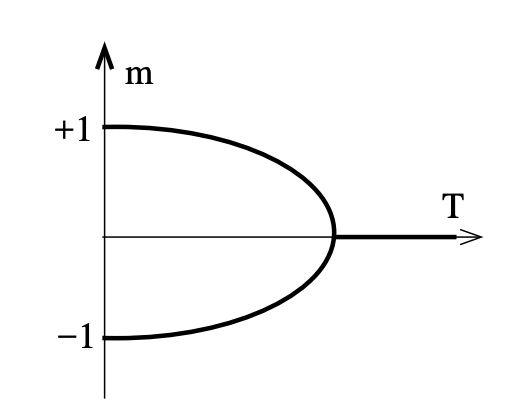
We can now consider the information manifold, parameterized by \(\beta\). For each point on the manifold (i.e. each distribution), we calculate a quantity \(E_\beta[m]\), for \(m(s)=\frac{1}{N}|\sum_i s_i|\). Note the absolute value.
For large \(\beta\), the distribution is dominated by two states, where all spins are up, and where all spins are down. In either case, we have \(m(s)=1\), so that \(E_\beta[m]=1\). However, as we increase the temperature, states such as the "chessboard" (alternating up and down spins) gain non-zero probability, and since these have \(m(s)=0\), we see \(E_\beta[m]\) decrease.
At small \(\beta\), all states have the same probability, and there are many more states with \(m(s)=0\), so that \(E_\beta[m] \to 0\). What is remarkable about the Ising model is that for large \(N\), the value of \(\beta\) for which \(E_\beta[m]=0\) for the first time tends towards a finite value.
This implies a non-analyticity of the function \(\beta \mapsto E_\beta[m]\) (it is always a fixed value, \(0\), after a certain point \(\beta^*\), but \(>0\) before, and this is not possible for an analytic function - there's a kink in the graph), and this is the characterizing property of the Ising model phase transition.
\(\beta^*\) is known as the critical point. As usual, we define \(T:=\frac{1}{\beta}\) as the temperature. Near the critical temperature, we find power law behavior, so for \(t := (T-T_c)/T_c\):
for \(\alpha, \beta, \gamma\) irrational constants that appear in a wide variety of models said to be in the same universality class as the Ising model.
Mean-field theories
(Mean-field) variational inference on the Ising model works as follows. As normal, we consider the manifold of identical independent distributions on the space (so \(q_H(s) = \Pi_iq_H(s_i)\)), with \(H\) the parameter, so that \(q_H(s_i) \propto e^{-\beta Hs_i}\).
We then vary \(H\) to maximize the lower bound on \(L \leq \log Z\):
We now exploit our mean field assumption:
\(L(H) = E_{s\sim q_H}[\log q_H] - E_{s\sim q_H}[\log \hat p] = E_{s\sim q_H}[-\beta H \sum_is_i - \log Z_H] - E_{s\sim q_H}[-\beta J \sum_{\langle i,j\rangle}s_is_j] = -\beta H NE[s_1] - \log Z_H + \beta J N\frac{1}{2}zE[s_1]^2\)
So that (at the minimum), now exploiting the properties of the derivative of the normalizing constant of the exponential family: \(0 = \frac{d}{dH}L(H) = -\beta NE[s_1] -\beta H N\frac{d}{dH}E[s_1] - \frac{1}{Z_H}\frac{d}{dH}Z_H + \beta J NzE[s_1]\frac{d}{dH}E[s_1] = -\beta H N + \beta J NzE[s_1]\)
This is sufficient to determine the effective "mean" field \(H\), by finding a value of \(m := E[s_1] = \tanh(\beta H) = \tanh(\beta JzE[s_1])\) that is self-consistent. Physicists often give a confusing justification for this choice of the \(H\) to do with eliminating fluctuations, but the above is clearer: we are introducing a simplifying constraint (namely, independence) and choosing the best distribution under those circumstances.
Exact solution of 2D Ising model
The fact that there is an exact solution to the 2D Ising model is valuable because it proves that the model exhibits phase transitions, and allows the calculation of critical exponents (against which approximate techniques can be compared).
Actually understanding the exact solution(s) is also valuable, since it involves fundamental ideas in statistical field theory.
Let \(N\) be the length of a side of the grid.
The transfer matrix method
This method is quite algebraic. We begin by expressing the normalization constant (aka partition function) \(Z\) as the normalization constant of a quantum system, i.e. as \(Tr(e^{-\beta H})\) where \(A^n = e^{-\beta H}\) is known as the transfer matrix (with \(n\) the length of the lattice). We then use standard techniques of many-body quantum physics.
To arrive at the desired form, we first consider a lattice of width \(N\) and height \(1\). We can view a configuration of this lattice as a basis element of a Hilbert space \(\bigotimes_i^N \mathbb{C}^2\). Concretely, let \(|s\rangle = |s_1\ldots s_n\rangle\) by an eigenvector of \(\sigma_3(i) := I_1 \otimes \ldots \otimes I_{i-1} \otimes \sigma_3 \otimes \ldots I\), so that \(\sigma_3(i)|s\rangle = s_i|s\rangle\). In other words, the state of the lattice at site \(i\) is specified by the eigenvalue of \(\sigma_3(i)\).
Then for a function \(b(K)\) (to be determined below), define:
so that we have:
so that with \(b(K) = \tanh^{-1}(e^{-2K})\), we recover the energy of the Ising model.
Note
\(b\) is an involution, and in fact represents the Kramers–Wannier duality : distributions parametrized by \(K\) and by \(b(K)\) on the manifold are (up to some factors) the same.
That makes \(V_3V_1\) function as a transfer matrix, in the sense that \(Tr((V_3V_1)^2) = \sum_s \sum_s' \langle s | V_3V_1 |s'\rangle \langle s' | V_3V_1 | s \rangle\) is a sum over all states of the Ising model for height \(3\) and so on for higher \(n\).
Note that our partition function is then also a time evolution of a quantum system.
Calculating \(Tr(V_3V_1)\) is difficult and requires us to rewrite the Pauli matrices as Majorana fermions (fermions following a Clifford algebra). After this, diagonalization is straightforward.
Under construction
Critical exponents
For a function \(f\), we write
to mean
These are the conventions:
Renormalization
Context
For any distribution \(p : Dist(A)\), in general we may have a function \(f : A \to B\), which we can pushforward to obtain a new distribution of type \(Dist(B)\). It is often the case that while \(f\) has no fixed points, \(f^* : Dist(A) \to Dist(B)\) does. A common example is Markov Chain Monte Carlo, where one finds a transition function \(f : S \to Dist(S)\), for a state space \(S\), but where \(f^* : Dist(S) \to Dist(S)\) has the stationary distribution as a fixed point.
In the setting of statistical field theory, we are dealing with distributions over functions of space or spacetime. Two interesting functions on these functions are (1) to drop frequencies below a cutoff (i.e. filtering, see the notes on Fourier analysis). Call this function \(g_s\), so that \(g_s(f(k)) = 1[k < s]f(k)\). Note that here, we express \(f\) in a frequency basis. Also note that if \(C(\Lambda)\) is the space of functions of type \(\R^n \to \R\) with frequencies less than \(\Lambda\), then \(g_s : C(\Lambda) \to C(s)\), and \(g_s^* : Dist(C(\Lambda)) \to Dist(C(s))\).
A second function on functions can be defined by \(h_s(f) = f \circ (x \maps xs)\). In that case, \(h_s^* : Dist(C(\Lambda)) \to Dist(C(\Lambda s))\).
The renormalization group is then the operation \((h_{\Lambda/s} \circ g_s)^* : Dist(C(\Lambda)) \to Dist(C(\Lambda))\). The fixed points of this operation are critical points.
Moreover, one can in various non-trivial cases calculate the stable manifold of the fixed point analytically, and recover extremely useful information about phase transitions.
Real space, discrete (Migdal-Kadanoff)
The simplest example of renormalization is illustrated with the 1D Ising model. Recall that the Ising model (aka Markov Random Field) has the form \(p({s}) = e^{\sum_{\langle i,j\rangle}Ks_is_j}\). Call \(I_{MRF}\) the space of distributions on the 1D lattice, parametrized by the choice of \(K\), so that \(Z(K)\) denotes a particular such distribution.
We are interested in some expectation, e.g. \(G(k, K) := \langle x_0x_k\rangle_K\). We then make three key observations:
- marginalization shouldn't affect the result, in the sense that \(G(32)\) could be calculate directly, or calculated after marginalizing out the odd sites
- the model we obtain after marginalizing out the odd sites lives on the same manifold \(I_{MRF}\) (if we assume the lattice is infinitely large), so is \(Z(f(K))\), for some \(f\). (Intuitively, the conditional independence structure of the model makes this clear: once we marginalize out sites \(1\) and \(3\), sites \(0\) and \(2\) will be dependent, but \(0\) and \(4\) will be conditionally independent given \(2\).)
- this act of marginalization therefore gives us a flow \(f\) on the manifold, and it will turn out that the fixed points are the critical points, i.e. where phase transitions happen.
Here are the details. The new model is given by:
We observe that \(\sum_{s_1 \in \{1,-1\}}e^{Ks_1(s_0+s_2)}\) is a function of \(s_0\) and \(s_2\) which is invariant under \(s_0 \mapsto -s_0, \quad s_2 \mapsto -s_2\), and since \(s_i^2=1\), we obtain: \(\sum_{s_1 \in \{1,-1\}}e^{Ks_1(s_0+s_2)} = e^{f(K)s_0s_2 + C}\)
We then get an equation for each choice of values for \(s_0\) and \(s_2\). In particular:
These can jointly be solved by \(e^{f(K)} = \sqrt{\cosh(2K)}\) and \(e^{C}=2\sqrt{\cosh(2K)}\), so \(\tanh f(K) = \tanh^2 K\).
As regards \(G\), note that then \(G(2n, K)= G(n, f(K))\), so that for \(G(n, K) = e^{-n/\xi(K)}\), we get:
This real-space approach to renormalization isn't particularly general; in the 2D Ising model for example, decimation introduces more complex relationships between variables, so the information manifold is no longer 1D, and instead we have terms \(K_1s_is_j, K_2s_is_js_ks_l\), and others.
Real space, continuous
Note
Most references aren't very clear on the fact that the space of distributions is a function of \(\Lambda\), and don't mention that we are performing a change of variables in the infinite-dimensional measure \(D\phi\), but without making these points explicit, the logic of renormalization is difficult to follow.
Our setting here is distributions over fields, i.e distributions over functions of space. Without (much) loss of generality, we consider distributions of the form:
where \(F\) is local. For example, we could have \(F=\int dx \phi(x)^2\) or \(\int dx a_1\phi^n + a_2\nabla^n\phi^m\ldots\). The coefficients \(a_i\) fully determine \(F\), so we can write a distribution as \(\rho(a)\).
We also want to specify the support of the distribution, in particular the band of frequencies allowed for a field in the support of the distribution. Call the maximum frequency \(\Lambda\) and write \(\rho(a, \Lambda)\) for a given distribution. Write \(Z(a, \Lambda) := Z(\rho(a, \Lambda)) := \int (D\phi) \rho(a, \Lambda)(\phi)\).
Note that fixing \(\Lambda\) specifies an information manifold of distributions \(\rho(\_, \Lambda)\) for which \(a\) are coordinates.
Our interest is in marginalizing out high frequencies (i.e. low length scales), to obtain a distribution \(Z(a'_i, \Lambda/b)\), and then rescaling back to the original support, to get a distribution \(Z(T(b)(a)_i, \Lambda)\), where the goal is to find \(T(b)\).
More concretely, let \(f_{\Lambda}(\phi)\) be a function which filters out frequencies above some \(\Lambda\), so that the pushforward \(Z(a'_i, \Lambda) = f_{\Lambda/b}\rho(a, \Lambda)\) is a distribution over fields with frequencies below \(\Lambda\). We then marginalize (i.e. pushforward by this map), to obtain a distribution \((f_{\Lambda/b}^*\rho(a, \Lambda)) \propto \int_{[\Lambda/b, \Lambda]}\rho(a, \Lambda)\).
This procedure is parametrized by \(b \in [1,\infty)\), and each \(a\) describes a point on the information manifold over fields, so what we have is a flow on the manifold. Certain fixed points of the flow correspond to critical points (i.e. points of phase transition), therefore our interest is in these points and their stability (i.e. the local linearization of the flow around these points).
Gaussian example
where the maximum frequency for functions \(\phi\) ranged over by the measure \(D\phi\) is \(\Lambda\).
In this case, we begin by marginalizing out frequencies above \(\Lambda/b\), to obtain a distribution \(Z(m', \Lambda)\).
for a constant \(\mathcal{N}\). This shows that in this case, \(m'=m\). We now need to pushforward the distribution by a map \(g_w(\phi) = (x \mapsto xb^w) \circ \phi \circ (x \mapsto xb)\), for \(w\) to be determined shortly, which scales the fields in the support. Note that the initial multiplication by \(b\) in real space amounts to a division by \(b\) in Fourier space, so that the support will contain functions that take frequencies up to \(\Lambda\).
To determine \(w\), observe that:
where \(\phi(x'b) = \phi(x) = b^{(2-d)/2}f(\phi)(x/b)\) and \(m' = mb^2\), so that \(w = \frac{d-2}{2}\).
This means that \(Z(g_w^*(f^*_{\Lambda/b}(\rho(m, \Lambda)))) \propto \int_\Lambda D(f(\phi))e^{-F_{m'}(\phi)} = Z(\rho(m', \Lambda))\),
so that
Note here that in changing variables from \(D\phi\) to \(D(g_w(\phi))\), we move from \(\Lambda/b\) to \(\Lambda\), as desired. Note also that the change of measure from \(D\phi\) should incur a Jacobian determinant, and without going into the theory of functional determinants, let us assume that this is a constant \(K\).
Since we are eventually concerned with derivatives of \(\log Z\) (which are the expectations of interest), the constant \(K\) is irrelevant. In this case, we find a fixed point for \(m = 0\) or \(m = \infty\).
In the more general case, things are much harder. This is because we can no longer trivially marginalize out the high frequencies, and instead have to resort to peturbative methods, e.g. via Feynman diagrams. However, calculations of this sort have been extremely important both in statistical physics and quantum field theory.
Landau theory
References
David Tong's notes are good as usual. Other resources often poorly motivate why the free energy can be viewed as a function of \(m\), which is both subtle and necessary to understand.
Note
It is expedient to use the Ising model as a running example, although Landau theory is a general technique.
The idea is to obtain the bifurcation diagram of a phase transition qualitatively (i.e. topologically correct) without computing the partition function explicitly.
Concretely, what we want to obtain is:
First, a definition: \(F(m, T) := -T\log \sum_{s|m}e^{-\frac{1}{T} H(s)}\), where \(\sum_{s|m}\) means the sum ranging over all configurations \(s\) with \(\frac{1}{N}\sum_i s_i = m\). Then:
In the case that the final integral is dominated by the minimum \(m^*\), we get \(Z(T) \approx e^{-\beta F(m^*, T)}\), so that \(F\) is, as suggested by the name, the equilibrium free energy.
Actually calculating \(F\) as defined here is usually intractable, but we can still make progress.
We first observe from the definition above that \(F\) has to respect certain symmetries. For the Ising model, \(F(m, T)=F(-m, T)\), as seen from the definition and the symmetry of the Hamiltonian. Further, we expect it to be analytic in \(m\), at least for a finite sum, so that in an expansion around the minimum (dropping the constant term):
The key fact is then that we know \(m^*\) must be \(0\) above the critical temperature.
But observe that the bifurcation diagram of the above polynomial (i.e. plotting the minimum \(m^*\) of \(F(m, T)\) as a function of \(T\)) shows two non-zero minima appearing precisely when \(r_0(T) \geq 0\). So we can deduce \(r_0(T) = a(T-T_c)\), at least close to \(T_c\).
Since \(m^*\) is minimal: \(0 = 2r_0(T)m^* + 4r_1(T)m^{*3} \Rightarrow m^*(T) = \pm \sqrt{\frac{2|r_0(T)|}{4r_1(T)}}\).
Landau-Ginzburg
We can generalize the above to a field. Let \(m : \R\times\R \to \R\), and write as above:
However now \(m\) is a function, so the final integral ranges over functions.
The simplest case is
For which \(p(m)\propto e^{-F(m)}\) is a (infinite dimensional) Gaussian. At and above criticality, we observe that for all \(x\), the marginal distribution \(m(x)\) must be \(0\), so at \(T=T_c\), \(\mu=0\).
Magnetic field and chemical potential
There is a relationship between magnetic fields and chemical potentials.
For example, \(H(n) = -J\sum_{\langle i,j \rangle}n_in_j\) would be a reasonable Hamiltonian for a lattice gas with no double occupation. If we assume that particles and energy can be exchanged with the bath (grand canonical ensemble) so that only mean energy and particle number is known, our distribution is:
But with the Ising model, we instead have \(H(s) = -J\sum_{\langle i,j \rangle}s_is_j - B\sum_is_i\). Only energy is exchanged (nothing moves), so our distribution is:
This is the same distribution, with a different interpretation. It suggests that to model a sort of thing with fixed number in a field (e.g. spins) is the same as modeling things with no fixed number without a field.
Spontaneous symmetry breaking
To say that the Ising model has a spontaneously broken symmetry is to say that in the limit
That is, in the limit of an infinitely large system (\(N \to \infty\)) and \(0\) temperature, an arbitrarily small magnetic field \(b\) will make the system choose either the all-spins-up or the all-spins-down state.
More generally, spontaneous symmetry breaking involves a system with a symmetry of the Hamiltonian that exhibits this kind of arbitrary sensitivity to perturbation, expressed by a non-commuting limit.
Examples of systems
There are a few systems which are ubiquitous in statistical physics, often because their thermodynamic properties can be calculated exactly, or because they exhibit interesting phenomena, like phase transitions.
Some principles these experiments demonstrate:
- it is usually possible to work in either the microcanonical or canonical ensemble, and derive the same results from either
- the equation of state (relationship between energy, entropy and volume) is often analytically derivable, and leads to experimentally testable predictions
Classical ideal gas
Let \(m\) be the mass of a single particle, and assume we have \(N\) non-interacting particles trapped in a volume \(V\). Let \(U\) be the potential function, so that \(U(q_i)=0\) if the particle is in the box, and \(\infty\) otherwise.
Fixed energy (microcanonical)
First choose some value of \(E\). Then:
where
where
Note that
where the volume of the d-sphere with radius \(R\) is \(Vol(S_{d,R})=\frac{\pi^{\frac{d}{2}}\sqrt{2mE}^{d}}{\Gamma(\frac{d}{2}+1)}\)
Since \(\Delta E\) is differentially small, we have:
Then:
And putting it all together:
Fixed temperature (canonical)
Since particles are independent, \(Z=\frac{Z_i^N}{N!}\)
Defining the thermal de-Broglie wavelength as:
with dimensions, where \(E=ML^2T^{−2}\), of \(\left(E^2T^2M^{-1}E^{-1}\right)^{\frac{1}{2}} = \left(ML^2T^{−2}T^2M^{-1}\right)^{\frac{1}{2}}=L\)
we then have:
(This is the usually seen as \(pV = Nk_BT\).)
Then note that energy per particle is then \(\frac{3}{2}T=\frac{\dot{q}^2}{2m}\), where \(\dot{q}\) is the momentum of a single particle, so that \(\sqrt{3Tm}=\dot{q}\)
But recalling that \(\lambda_{dB}=\frac{h}{p}\) is the de Broglie wavelength, we see why \(\lambda\) is called the thermal de Broglie wavelength, since it is, up to a constant, the wavelength of the average particle.
Equation of state
The equation of state for the ideal gas is known as the Sackur-Tetrode formula. We can derive it as follows:
Now note that \(\pd{}{T} N\left(\log \left(\frac{V}{N\lambda^3}\right) + 1 \right) = -N\pd{}{T}\log(\lambda^3)=-N\pd{}{T}\log\left(\frac{2\pi\hbar^2}{mT}\right)^{\frac{3}{2}}=\frac{3}{2}N\)
so
Quantum Harmonic Oscillator
The state space is \(\mathbb{N}\), the natural numbers, with \(E(n)=(n+\frac{1}{2})\hbar\omega\). Then:
Proceeding in the normal fashion, we obtain as energy and heat capacity:
At low \(T\), we can see that \(E\) becomes increasingly constant (in \(T\)), but at high \(T\), becomes linear in \(T\) (you need to consider the locally linear region near \(\beta=0\), since otherwise we get division by \(0\). This is the thermodynamic behaviour predicted by the corresponding classical model.
Further note that \(\omega = \sqrt{\frac{k}{m}}\), so similar remarks hold for oscillators with a strong spring constant, for example.
Note: one example of a physically useful consequence of this: a gas of diatomic molecules should have vibrational energy from the molecules (which are harmonic oscillators), but if their spring constant is high enough relative to the temperature of the system, we can treat them as frozen. More generally, we get locking of certain degrees of freedom. This explains why macroscopic systems have lower energy than classical statistical mechanics predicts, and similarly the heat capacity of solids (lattices of harmonic oscillators) was overestimated classically. Another example is a vibrating string. If each complex exponential (harmonic oscillator) in its Fourier series had energy equal to the temperature, the total energy would be unbounded. We need instead to say that the high frequency oscillators have exponentially small temperature.
A crystal
For simplicity, assume we have a 1D lattice (same ideas apply in 3D). The configuration of the lattice can be represented by a vector \(\textbf{q}\), giving the displacement from equilibrium of each atom. Moreover assume periodic boundary conditions so that \(q_{N+1}=q_N\). Kinetic energy is then straightforward, namely \(\sum_i^N \frac{p_i^2}{2m}\).
The problem is the potential, which could be enormously complex. What we can do is to consider the low temperature case, where displacements are small, and so a Taylor expansion is justified, with:
We can then diagonalize \(H=\left(\nabla^2U|_{q_0} \right)\) to obtain a new formula for \(N\) independent oscillators, which allows us to express the partition function as a sum of independent harmonic oscillators (either quantum or classical).
The next step is to approximate the sum by an integral, which requires us to provide a density \(\sigma(\omega)d\omega\) over frequencies for our harmonic oscillators. Notice that this is a continuum approximation of the solid.
The Debye model provides one choice of \(\sigma\).
The much simpler Einstein model of a solid, which qualitatively captures the fact that the heat capacity drops with temperature, is to treat a solid as a set of \(3N\) harmonic oscillators, all sharing the same \(\omega\).
Gas with quantized energy levels
(These lecture notes were helpful here)
Suppose that we have \(N\) particles, energy levels denoted \(e(i)\), and number of particles per level denoted \(R(n_i)\) (in a full state of the system \(R\)). Then \(N=\sum_ie(i)R_n(i)\) in that state. Assume that temperature (and chemical potential) are fixed.
Then under different assumptions we obtain different values of \(Z\), and can proceed from there.
With distinguishable particles (Maxwell-Boltzmann statistics)
If the particles are distinguishable, we have:
where \(\xi = \sum_ie^{-\beta e(i)}\)
Then
With indistinguishable bosons with no fixed number (Bose-Einstein statistics)
Here we have to use the Grand Canonical Ensemble, namely:
with \(R(E) = \sum_ie(i)R(n_i)\) and \(R(N) = \sum_i R(n_i)\):
So
and
Similarly: \(\langle n_j \rangle = \frac{1}{e^{\beta(e(j)-\mu)} - 1}\)
Note that since \(\forall j: \langle n_j \rangle \gt 0\), we have \(\forall j: E_j\gt \mu\). In particular, as \(\mu\) approaches the lowest energy \(E_0\), \(\langle n_0 \rangle \to \infty\) and so almost all of the particles reside in the ground state. This is Bose-Einstein condensation, and leads to weird macroscopic effects of quantum behaviour.
With indistinguishable fermions with no fixed number (Fermi-Dirac statistics)
Now assume the particles are Fermions. Proceeding in the same fashion, but summing \(n_i\) up to \(1\), not to infinity, in order to respect the Pauli exclusion principle for Fermions, we obtain:
This is a useful model of electron and hole density in semiconductors. Note that \(\langle n_j \rangle \leq 1\), as we would want.
Two spin system
A state \(s\) is an array of \(N\) Booleans, and the energy is \(E=\epsilon\cdot N_T(s)\), where \(N_T(s)\) is the number that are true (or spin-up, if you prefer).
Note that in this system, we have fixed number and volume, so don't have to worry about those.
Two Spin System: Microcanonical Ensemble
The microcanonical ensemble is binomial, and so the entropy is \(0\) at \(E(s)=N_T(s)\epsilon=0\).
Using Stirling's approximation, entropy at \(E=\epsilon N_T\):
Symbolically solving, to save effort, and working in units where \(k_B=1\), we calculate \(S(E)\) and \(E\) in terms of \(T\):
which forms roughly a semicircle when graphed (\(S\) on y-axis, \(E\) on x-axis). From this, we see that temperature is negative when \(E \gt \frac{N_T}{2}\). Further, negative temperatures are hotter than positive ones, in the sense that heat flows from a system with negative temperature to a system with positive temperature. To see this, suppose we place system \(1\) with positive temperature next to system \(2\) with negative temperature. \(dS \gt 0\), so
\(\frac{dS_1}{dE_1} = \frac{1}{T_1} \gt 0\) and \(\frac{dS_2}{dE_2} = \frac{1}{T_2} \lt 0\)
Then energy must be added to system \(1\) to increase energy, and removed from system \(2\).
Schottky anomaly
Inverting the equation for \(S(E)\) to obtain \(E(S)\), we see that:
Heat capacity is defined as:
Graphing this shows a non-monotonic curve. This non-monotonicity is known as the Schottky anomaly, anomalous relative to the monotonic heat capacity for many types of systems.
Two Spin System: Canonical Ensemble
We calculate:
Note that this agrees with the same result obtained from the microcanonical ensemble after a Legendre transform.
Classical Harmonic Oscillator
Microcanonical ensemble
\(1 = \int d^{6N}\mu \rho = C'\cdot A\), for \(A=\int_{E \leq \sum_{i}^{3N}\frac{p_i^2}{2m}+\frac{kq_i^2}{2}\leq E+\delta E} dq_1...q_n,p_1...p_n\)
To evaluate this integral, we can note that for \(\tilde{\Omega}(E)=\int_{\sum_{i}^{3N}\frac{p_i^2}{2m}+\frac{kq_i^2}{2}\leq E} dq_1...q_n,p_1...p_n\), we have that \(A=\tilde{\Omega}(E+\delta E)-\tilde{\Omega}(E)\).
\(\tilde{\Omega}(E)\) is can be obtained by the formula for the volume of a sphere, and a change of variables to \((\frac{p_1}{\sqrt{m}}...\frac{p_n}{\sqrt{m}},\sqrt{k}q_1...\sqrt{k}q_n)\), which incurs a Jacobian determinant of \((\frac{m}{k})^{\frac{3N}{2}}\). In particular:
So in the limit of small \(\Delta E\), we have that \(\frac{A}{\Delta E}=\frac{\partial A}{\partial E} = \sqrt{\frac{m}{k}}^{3N}\frac{\pi^{3N}(2E)^{3N}}{\Gamma(3N+1)}=\frac{6N\sqrt{\frac{m}{k}}^{3N}\pi^{3N}(2E)^{3N-1}}{\Gamma(3N+1)}\)
Then, again in the limit of small \(\Delta E\), \(C'=\frac{1}{\Delta E}\frac{\Gamma(3N+1)}{6N\sqrt{\frac{m}{k}}^{3N}\pi^{3N}(2E)^{3N-1}}\)
Canonical ensemble
Let's consider a single, 1D classical harmonic oscillator. I use \(\mu\) to denote a point in phase space, with coordinates \((p,q)\). Assume units where \(k_B\) is \(1\).
where \(\omega\) is \(\sqrt{\frac{k}{m}}\), which is the frequency of the oscillator.
So \(E = -\frac{\partial \log Z(\beta)}{\partial\beta} = \frac{1}{\beta} \Rightarrow E = T\)
This means that for any spring constant, the oscillator is equal to the temperature. This turns out not to be the correct model for nature: it turns out that at low temperatures and high spring constants, heat capacity decreases. Explaining this requires quantum mechanics.
Kinetics
Kinetics is the application of actual mechanics to obtain physical behaviors of large systems. So for example, you could take the Maxwell speed distribution of particles in an ideal gas, and look at their collisions with the sides of a box, for example, to work out how much force they should impart, and thus what the pressure is.